


Speech recognition works by converting sound into digital samples, transforming those samples into acoustic features, using a neural network acoustic model to predict phoneme probabilities, and applying a language model to decode the most likely word sequence. Modern systems like OpenAI Whisper and Conformer-based models achieve word error rates below 10 percent on clean audio. If you are building voice features, VideoSDK's real-time transcription brings this pipeline into live video and audio rooms with sub-second latency.
You ask your voice assistant for the weather in "Tour-in," and it cheerfully books you a table at a restaurant in Turin. Anyone who has built a voice feature knows that moment: the model heard the sounds correctly but understood the world wrong. Understanding why that happens means understanding the full pipeline behind automatic speech recognition (ASR).
So, how does speech recognition work? This question matters whether you are a developer wiring a speech-to-text API into a product, a product manager evaluating transcription vendors, or an engineer deciding between edge and cloud inference. By the end of this article, you will understand the five-stage flow from raw sound to readable text, the modern model families powering it, and the production realities that separate a demo from a shippable feature.
How Does Speech Recognition Work: An Overview
Speech recognition is defined as the process of converting spoken audio into text by mapping acoustic signals to linguistic units. It works by capturing audio, extracting acoustic features from that audio, predicting which speech sounds are present at each moment, and then decoding the most probable sequence of words given both the acoustic evidence and the rules of the language.
At the highest level, the pipeline has three phases: audio capture and digitization, acoustic modeling, and decoding with a language model. Each phase hides significant engineering detail. The digitization phase decides how faithfully sound is represented. The acoustic modeling phase decides how sounds map to phonemes. The decoding phase decides how phoneme probabilities become actual words, resolving ambiguities like "four" versus "fore" using context.
The rest of this article walks through each stage in order, then covers post-processing, production pitfalls, and where the field is heading in 2026.
From Sound to Digital Numbers: Sampling and Framing
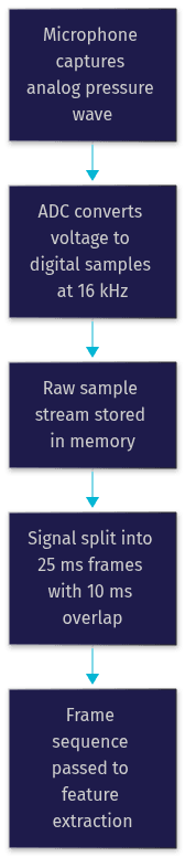
Every speech recognition system begins with a physical pressure wave. A microphone converts that wave into an analog voltage, and an analog-to-digital converter (ADC) measures the voltage thousands of times per second. Each measurement is a sample, and the sampling rate determines how much acoustic detail survives digitization.
Most modern ASR systems use a 16 kHz sampling rate, which captures frequencies up to 8 kHz. That range covers the bulk of human speech energy, since most phoneme-distinguishing information lives between roughly 300 Hz and 3,400 Hz. Telephony audio at 8 kHz loses the higher frequencies, which is why phone-call transcription is noticeably harder than studio-quality audio.
Once digitized, the audio is chopped into short overlapping windows called frames, typically 20 to 25 milliseconds long, with each frame overlapping the previous one by about 10 milliseconds. The overlap matters: speech sounds blur across boundaries, and overlapping windows ensure no transition between phonemes falls into a gap between frames.
There is a storage trade-off here worth noting. A 16 kHz, 16-bit mono recording consumes roughly 32 kilobytes per second, or about 115 megabytes per hour. For long-form batch transcription, teams routinely downsample or compress audio before upload, which can degrade accuracy if the compression is aggressive.
Turning Raw Waveforms into Meaningful Features
Raw audio samples are nearly useless to a machine learning model. A waveform is just a long sequence of air-pressure measurements, and the information that distinguishes an "s" from a "sh" lives in the frequency content, not in individual samples. Feature extraction converts each frame into a compact numerical description of its frequency content.
The workhorse of this stage is the spectrogram, produced by applying a Short-Time Fourier Transform (STFT) to each frame. A spectrogram is a time-frequency heat map: time runs along the horizontal axis, frequency along the vertical axis, and color intensity shows how much energy exists at each frequency at each moment. Read a spectrogram of the word "cat" and you can literally see the burst of the "k," the steady hum of the vowel, and the hiss of the "t."
Most systems go one step further and convert the spectrogram into mel-frequency cepstral coefficients (MFCCs). The mel scale mimics how human hearing perceives pitch, giving finer resolution at lower frequencies where speech information is densest. MFCCs compress each frame into a few dozen coefficients, discarding irrelevant variation like overall loudness while preserving the spectral shape that identifies phonemes.

Feature normalization and noise reduction happen at this stage too. Normalization adjusts each utterance so that a quiet speaker and a loud speaker produce comparable feature values. Noise reduction, often a small neural network itself, suppresses background hiss before features are computed. Voice activity detection (VAD) also runs here, marking which frames contain speech so the acoustic model never wastes computation on silence.
Acoustic Modeling: From Features to Phonemes
The acoustic model is the heart of any speech recognition system. Its job is to look at the feature vectors, frame by frame, and output a probability distribution over speech sounds for every frame. Those speech sounds are phonemes, the smallest units that distinguish words, such as the three phonemes separating "cat" from "bat."
Historically, this job belonged to Gaussian Mixture Model and Hidden Markov Model (GMM-HMM) combinations. The HMM handled the fact that phonemes stretch and compress in time, while the GMM estimated feature probabilities. These systems worked but plateaued in accuracy, largely because GMMs could not fully exploit the correlations between spectral features.
Modern systems replaced this stack with deep neural networks. Recurrent architectures with LSTM units modeled temporal context directly, and today's state of the art belongs to models like the Conformer, which combines convolutional layers that capture local acoustic detail with transformer attention that captures long-range context. OpenAI's Whisper, trained on roughly 680,000 hours of multilingual and accented audio, uses an encoder-decoder transformer and remains the most widely used open-source ASR model as of 2026.
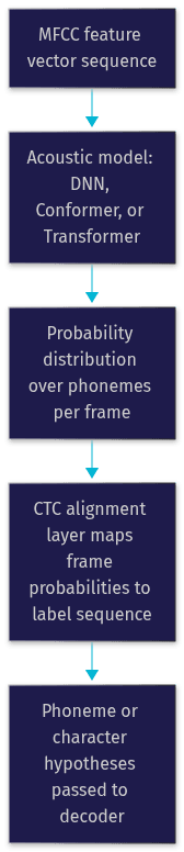
One problem dominates acoustic modeling: the alignment problem. Speech does not come labeled with timestamps saying when each phoneme starts and ends, and speakers vary wildly in pace. Connectionist Temporal Classification (CTC) solved this elegantly. A CTC-trained model outputs one prediction per frame plus a special blank symbol, and the training process learns to collapse repeated predictions into a single label without needing frame-level annotations. CTC is the reason streaming ASR works: a CTC model can emit partial hypotheses as frames arrive rather than waiting for the utterance to finish.
A pronunciation dictionary traditionally mapped phonemes to words, though modern end-to-end models often predict characters or subword units directly, learning pronunciation implicitly from data. This removes the dictionary bottleneck for new words and domain jargon, at the cost of needing more training data.
Language Modeling and Decoding
Acoustic output alone is ambiguous. The sounds in "recognize speech" and "wreck a nice beach" are nearly identical, and no acoustic model can distinguish them with certainty. The language model (LM) resolves this by scoring how plausible a candidate word sequence is in the language, based on the statistics of how words follow one another.
Older systems used n-gram language models, which count how often word sequences appear in a large text corpus. They are fast and compact but cannot generalize to word combinations they have never seen. Modern decoders use transformer-based neural language models, the same architecture family behind GPT-style models, which generalize far better and can be tuned to a specific domain like medical dictation or legal transcription. Shallow fusion is a common technique for combining an acoustic model's output distribution with a language model's scores during decoding.
Decoding itself is the search for the best word sequence given both the acoustic and language scores. Greedy decoding simply picks the highest-scoring token at each step, which is fast but error-prone. Beam search keeps the top several candidate sequences alive at each step and selects the best complete hypothesis at the end. The classic Viterbi algorithm performs the equivalent search over HMM state sequences and still underpins many production systems.
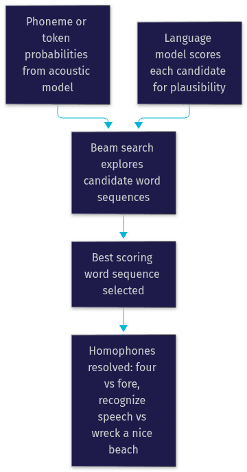
This is exactly where the Turin weather request went wrong. The acoustic model heard the sounds fine; the language model, lacking context about the user's travel plans, ranked a restaurant booking as the more probable interpretation. In practice, teams fix this by biasing the language model toward domain vocabulary, a technique called contextual biasing.
Post-Processing and Real-World Enhancements
Raw decoder output is lowercase, unpunctuated text with no speaker boundaries. Post-processing turns it into readable transcripts. Text normalization converts spoken forms into written forms, so "twenty twenty-six" becomes "2026" and "dot com" becomes ".com." Punctuation and capitalization models, usually small transformers trained on paired text, insert commas, periods, and sentence casing. Inverse text normalization handles the reverse direction when the transcript feeds a downstream system.
Voice activity detection and endpointing deserve special attention in voice interfaces. Endpointing is the decision of when the user has finished speaking and the system should respond. Cut off too early and the system truncates the utterance; wait too long and the interaction feels sluggish. Production systems typically use a silence threshold of 500 to 800 milliseconds, tuned against measured user behavior.
When multiple people speak, speaker diarization segments the transcript by who said what, typically by clustering speaker embeddings extracted from the audio. This is essential for meeting transcription and call analytics.
Finally, there is the deployment question: edge or cloud. On-device inference offers privacy and works offline, but model size is constrained, so accuracy typically trails cloud models. Cloud inference offers the largest models and easiest updates, but adds network latency and raises data-handling obligations. Many production systems run a small on-device model for wake words and VAD, then stream audio to a larger cloud model for full transcription. VideoSDK's real-time transcription takes this hybrid approach inside live rooms, so a video call can carry live captions without the application team building the ASR pipeline itself.
Common Pitfalls and Production Tips
Most production speech recognition failures trace back to three causes: noise, low-quality audio, and mismatch between training data and real users.
Noisy environments break acoustic models trained on clean studio audio. The standard fix is data augmentation during training, mixing in background noise, room reverberation, and codec artifacts so the model learns robustness rather than fragility. Accent and dialect mismatch is the same problem in disguise, and the cure is the same: diverse, multilingual, accented training data, which is precisely why Whisper's 680,000-hour corpus performs so well across accents.
For low-bandwidth devices, adaptive gain control and aggressive VAD reduce wasted computation, and quantized on-device models shrink memory footprint with modest accuracy cost. In production, monitor two metrics continuously: word error rate (WER), the percentage of words the system gets wrong against a reference transcript, and end-to-end latency. A WER below 10 percent is generally considered production-grade for clean audio, while real-time streaming interfaces typically target partial-transcript latency under 300 milliseconds.
Future Directions in Speech Recognition
Three trends are reshaping the field as of 2026. First, multimodal speech recognition combines audio with visual input, lip-reading from video to improve accuracy in noisy environments, a natural fit for video-calling platforms. Second, large language models are being fused directly into ASR decoding, with LLM-powered rescoring and even end-to-end speech-to-LLM architectures that skip explicit text intermediates. Third, privacy-preserving techniques like federated learning let models improve from user data without that data ever leaving the device.
On-device ASR is also maturing fast, driven by quantized transformer models and dedicated neural accelerators in modern phones and laptops. Meanwhile, independent leaderboards like Artificial Analysis's Speech Arena now benchmark ASR providers on real conversational audio, giving engineers vendor-neutral data instead of marketing claims when choosing a speech-to-text engine.
Definitions Glossary
Frame: A short overlapping window of audio, typically 20 to 25 milliseconds, that the system analyzes as a single unit so phoneme transitions never fall between analysis windows.
Spectrogram: A time-frequency heat map of audio produced by the Short-Time Fourier Transform, showing how energy at each frequency changes over time.
MFCC: Mel-frequency cepstral coefficients, a compact set of features per frame that mimics human pitch perception and preserves the spectral shape that distinguishes phonemes.
Phoneme: The smallest unit of sound that distinguishes one word from another, such as the single phoneme difference between "cat" and "bat."
Acoustic model: The neural network that maps audio features to probability distributions over speech sounds for every frame.
CTC: Connectionist Temporal Classification, a training method that lets models align audio frames to output labels without frame-level annotations, enabling streaming transcription.
Language model: A model that scores how plausible a word sequence is, resolving acoustically ambiguous phrases like "recognize speech" versus "wreck a nice beach."
VAD: Voice activity detection, the component that marks which audio frames contain speech so the system skips silence and detects when a user stops speaking.
Key Takeaways
- Speech recognition works through a five-stage pipeline: digitization, feature extraction, acoustic modeling, language-model decoding, and post-processing, and a weakness in any stage degrades the final transcript.
- CTC training is what makes real-time streaming transcription possible, letting models emit partial hypotheses as audio frames arrive instead of waiting for the utterance to end.
- The language model, not the acoustic model, resolves homophones and near-homophones, which is why contextual biasing toward domain vocabulary is one of the highest-impact production improvements.
- Production success depends on monitoring word error rate and latency, and on training or fine-tuning with noisy, accented, real-world audio rather than clean studio data.
- If you are adding live transcription to a video or audio product, VideoSDK's real-time transcription handles the ASR pipeline inside live rooms so your team can focus on the application, not the infrastructure.
Conclusion
Understanding how speech recognition work plays out in practice, from a 16 kHz sample stream to frames, MFCC features, phoneme probabilities, and a beam-searched word sequence, gives you the vocabulary to diagnose failures instead of guessing at them. When a transcript is wrong, you can now ask whether the problem was audio quality, feature extraction, the acoustic model, or the language model's context, and each answer points to a different fix.
The best next step is hands-on: run an open-source model like Whisper on a sample of your real users' audio, measure the word error rate yourself, and compare it against a managed API. If your product involves live conversations, try VideoSDK's real-time transcription inside a video calling room and see live captions working in minutes. You can start free at app.videosdk.live.
What speech-recognition challenge are you tackling, noisy call centers, accented users, or real-time captions? Drop a comment, I'd love to hear what you're building.
Free $20 Balance for AI Voice Agents & Video Calls
FAQ